Reconstruction of a Periodic Wire Mesh Pattern
from a Microscopic Image of Paper
03/09/2000
Author: Jason Plumb
Table of Contents
Abstract
Introduction
[Technical Approach](#tech approach)
[Transform to Frequency Domain](#trans to FFT)
[Recreation of Mesh Configuration](#recreate mesh)
Conclusions
[Appendix A: Software Manual](#appendix a)
[Appendix B: Software Source Code](#appendix b)
Abstract
This paper describes the design and implementation of a software program that can be used to reconstruct the periodic wire mesh pattern from a microscopic image of paper. The software uses a two dimensional Fourier transform to display the frequency spectrum of the input image. A pair of complex conjugate poles can then be selected for use in computing the inverse Fourier transform of the frequency spectrum. Using the selected frequency components, the software then reconstructs the original wire mesh pattern in the spatial domain. The software includes a user interface and is designed to run on Windows operating systems.
Introduction
In the paper making process, a combination of wood pulp and water (called "slurry" in the paper manufacturing industry) is applied to a a fine metal mesh. The slurry and metal mesh combination is then run through a series of processes (including pressing and heat drying) to remove the water from the wood pulp. When the water removing processes are complete, the wood pulp is eventually removed from the mesh and a paper product results.
At the microscopic level, the paper retains a slight imprint of the original wire mesh. When the microscopic image is viewed by the human eye, the mesh configuration is hard to distinguish. The original configuration of the wire mesh can, however, be recreated by applying image processing techniques. Because the wire mesh pattern that remains on the paper is periodic, it has frequency components that can be easily viewed in the Fourier transform of the image. The frequencies that comprise the mesh imprint can thus be used to create an image that closely models the original mesh pattern.
This approach has been used in the past in an attempt to identify the manufacturer of a specific type of paper.
Technical Approach
The software developed for this project uses a Windows graphical user interface do display images for the user. All images used by this software must be in Portable Gray Map (PGM) format. When an image is loaded from disk, it is immediately displayed in the user interface. The program utilizes the Cpgmfile class to simplify operations necessary for dealing with PGM files. The class contains methods for loading PGM files from disk, saving PGM files to disk, and obtaining specific image attributes (such as image height, width, and number of gray levels).
Although the program created for this project can operate on any PGM file, its primary purpose is to analyze a microscopic image of paper. The specific image in question is shown below in Figure 1.
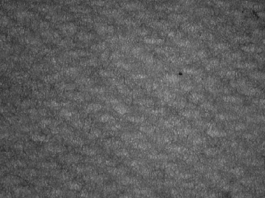
Figure 1: Original Input Image
When the image is loaded by the user, an off screen device context and associated off screen bitmap are created to store the image content. A handler for the WM_ERASEBACKGROUND message performs the operations required to draw the image to the screen.
Although one can clearly see that there is a repeating pattern somewhere in the image, it remains difficult to discern its details with the human eye.
Transform to Frequency Domain
When the user presses F2 (or chooses View->Fourier Transform from the menu), the program begins creating the frequency representation of the original image. The doViewFT() function is responsible for performing this operation. Because of the fact that an efficient 1-D discrete FFT algorithm was provided in advance, the program uses the separability property of the 2-D discrete Fourier transform.
The separability property allows a 2-D Fourier transform to be performed via multiple executions of 1-D Fourier transforms. The doViewFT() function calls the four1 function once for each row. Each pixel value in the input row is multiplied by (-1)(x+y) prior to the transform. This technique causes the frequency spectrum in the output image to have its origin centered appropriately. Each value in the resultant row is then multiplied by the row width, and stored in memory for later use.
After all rows have been processed by the four1 function, a DFT is performed for each column. The transformed column is stored back into the memory buffer. When all columns have been processed, the memory buffer contains the final Fourier transform of the input image.
In order to display the image to the screen, the magnitude of each point must be calculated. This is performed by computing sqrt(rere + imim), where _re _is the real component and im is the imaginary component. Usually, a frequency spectrum image is compressed and contains less information than desired. To overcome this compression, the software uses a logarithmic scaling factor when creating the image of the spectrum. The function 45*log10(1 + mag) (where mag is the pixel magnitude and 45 is the scaling constant) provides this scaling. The frequency spectrum of the original image is shown in Figure 2.
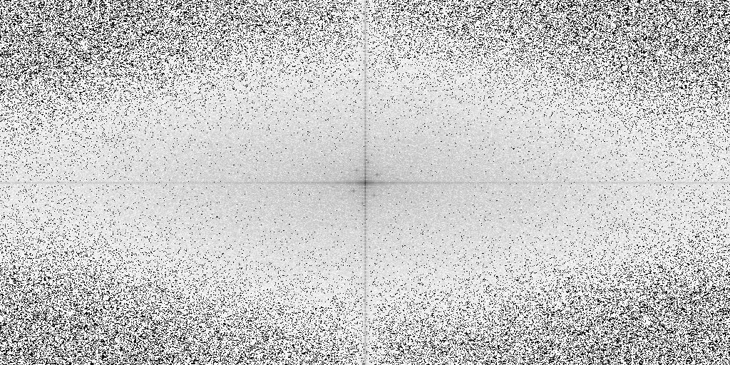
Figure 2: Frequency Spectrum of Original Input Image of Paper
One notices immediately that there are several small dark regions near the origin. These relatively low frequency components correspond to the primary frequency components of the wire mesh.
Recreation of Mesh Configuration
In order to recreate the wire mesh pattern from the Fourier display, the user must choose two points to be used in the inverse transformation. Once these points are chosen, the inverse transform can be created by pressing F3 (or choosing View->Overlay) from the menu.
The doViewOverlay function is responsible for computing the inverse Fourier transform of the previously selected points. The function first creates a memory buffer to hold the converted values. It then loops through the array of user-selected points and inserts the corresponding values (both real and imaginary parts) from the frequency representation. Similar to the forward transform (described above), the doViewOverlay function uses the separability property and calls the four1 function once for each row in the memory buffer. The transformed rows are placed back into the memory buffer for use in computing the column transforms. Each column is extracted from memory and placed into a column array. Once each column array has been processed by the four1 function, it is then placed back into the memory buffer.
Because the memory buffer now contains the 2-D discrete inverse FFT representation of the frequency plot, it can be displayed on the screen. This is accomplished by computing the magnitude of each point and scaling by a factor of 1/100. It should be noted that this scaling factor was somewhat arbitrarily chosen by the author, and other scaling factors will likely yield different results. It should also be noted that the resulting spatial domain image is clipped to the original image width and height. Because the mesh pattern is periodic with low frequency, this has little effect on the final display image.
The recreation of the mesh pattern from the original paper image is shown in Figure 3.

Figure 3: Reconstructed Wire Mesh Pattern After Inverse 2-D FFT
Results
By observing the image in figure 3, one can clearly see the recreation of the original wire mesh pattern. The grid appears to be angled, as thought the image were not taken perpendicular to the paper surface. One also notes that each grid cell appears to be rounded, and not completely rectangular. It is the author's opinion that the original mesh configuration may have used a hexagonal grid pattern.
When compared with the original image, Figure 3 seems to closely match the mesh configuration. It is believed that the figure above accurately displays the periodic pattern nested within the original image.
Conclusions
In conclusion, it can be said that the software created for this project performs well in recreating the wire mesh pattern. Although this is true, there are several aspects of the program's operation that could use improvement.
First, the program is limiting in that it restricts the number of components that may be selected when viewing the frequency spectrum. If the user does not select 2 points, the inverse Fourier transform cannot be computed. The software could be used in other applications and made into a generalized image analysis tool, if the number of frequency points were not limited in this manner. Ideally, an arbitrary number of points could be selected for use in the transform.
Next, it should be noted that the final spatial domain output image of the wire mesh pattern is somewhat difficult to look at with the humn eye. Additional processing of the output image would create a more pleasant result. Specifically, a DC term could be added to offset the purely periodic image. Additional techniques, such as threshholding, could also be applied to create a more pleasant output image.
Another issue of significant importance is the issue of speed. Because the program uses the FFT algorithm, it does perform quite well. However, there are a few specific changes that could be implemented to improve the program's speed. When performing the row operations used in performing both the FFT and the inverse FFT, each row is copied into a temporary row buffer, and the temporary buffer is passed to the four1 function. This step is actually quite unnecessary. The rows should be passed to the four1 function in-place, so that additional copies are not required. The overhead in copying to and from the temporary row buffer has a significant effect on the speed performance of the application.
The program also does not cache each image when switching between view modes. That is, when the user switches to a different view of the image, the previous image memory is discarded. Although this has the benefit of having a lower memory overhead, it still slows down the program's operation. An alternative approach would be to cache all memory for each image to allow more rapid switching between views.
Finally, the program could have a better means of qualifying the accuracy of the final mesh recreation. If the original image and final mesh recreation could be viewed side by side on the same screen, the user could get better idea of how accurate the recreation is. The author's original intention was to overlay the recreated mesh pattern on top of the original input image. Unfortunately, this feature has not been properly implemented. If the overlay could be viewed with a variable (user configurable) transparency, it could let the user see just how closely the recreation models the input.
Appendix A: Software Manual
This appendix provides a brief overview of the software usage.
Installation: To install the software, simply copy the executable program to any available location using the command prompt or Windows explorer. There are no additional support files that must be copied. The program is able to run as a stand alone executable.
Execution: The program can be started from the command line by typing "fourier" and pressing
Usage: When the program is first started, a blank window is displayed. To open an input image for processing, the user may choose File->Open from the menu, or press CTRL-O. While the image is being loaded for display, the cursor will momentarily change to an hourglass.
Once the image has been loaded, the Fourier spectrum can be displayed by pressing F2 or choosing View->Fourier from the menu. Again, the hourglass will momentarily change to an hourglass while the operation is being performed. After the operation has completed, the spectrum will be displayed with the horizontal and vertical axis in red. At this point, the user must select the two frequency components of interest before continuing. It should be noted that if the program was started with the "-hc" parameter, this operation will be completed automatically.
Frequency components are selected by clicking the associated points on the screen. When a point has been selected, it's 4-connected components will be highlighted in blue. Extreme care must be taken in choosing the frequency components. If an error is made, the file must be closed and re-opened. To ensure accuracy in selecting frequency components, the mouse location can be displayed in the lower right hand corner of the window by holding down the SHIFT key while moving the cursor. It should also be noted that when a point is selected, the program will automatically select (highlight) its complex conjugate partner.
After the points of interest have been selected, the user can convert the image back into the spatial domain by pressing F3 (or choosing View->Overlay from the menu). Again, the cursor turns into an hourglass while the operation is being performed. When complete, the spatial representation of the previously selected frequency components will be displayed on the screen.
While any image is displayed on the screen, the user may save it to disk by choosing File->Save As from the menu (or pressing CTRL-A). If the user selects an existing file when specifying a filename, he will be prompted before the file is overwritten. The file will be saved in PGM format.
Appendix B: Software Source Code
The software provided here has been designed to be compiled with Microsoft Visual C++ version 6.0.
- pgmfile.h, pgmfile.cpp - Helper class for dealing with PGM files
- fourier.h, fourier.cpp - Main application implementation files
- four1.h, four1.cpp - 1-D FFT routine files (from Numerical Recipes Software)
- fourier.exe - Executable program file
Images:
- proj2.pgm - Original image of paper